1. INTRODUCTION

This paper deals with the reconstruction of a building, starting from a point cloud. The test example is the China Central Television tower, located in Beijing.

The construction began in September 2004 on the 20 hectare site of an abandoned motorcycle factory in Beijing’s new Central Business District and was completed by Office for Metropolitan Architecture (OMA) in August 2008.

We had to solve the following problems: the structure is modeled by points, acquired from pictures available on the web and in architectural literature, and defined only by their three orthogonal Cartesian coordinates, without any other distinction, as shown in the following image, extracted by the data set.

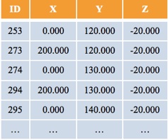
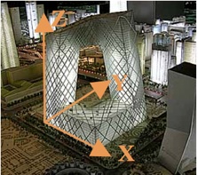
Figure 1.  Extract of input data set                                       Figure 2. Reference system adopted

The shape of this building is:

1. •non-stellar: starting from one point, to reach all the other points, it may be necessary to go outside the structure;
   

2. •concave
   

3. •multi–connected: this means that there is a hole.
   

The structure is composed of sowns and vertical or almost vertical walls (treated as chains).

The imposition of an arbitrary reference system is needed to remove the uncertainty of the origin, orientation and scales. The origin is placed on the left hand side, the axes as right-hand coordinate system and 1 m in reality is 1 unit in the data set.

The results will be given in the same reference system in which the coordinates are provided. The first 3D plot shows the structure represented by the point cloud.

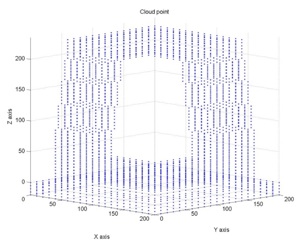
Figure 3.  3D plot of point cloud

3D reconstruction uses a sequence of procedures because it is almost impossible to use a single algorithm. The 3D model could be done in different ways, here the authors present the way chosen.

2. VOXEL

A voxel is an element of the total volume, representing a value on a regular grid in 3D space. The position of a voxel is inferred based upon its position relative to the other voxels.

The first procedure is devoted to checking the data set, to detecting the minimums and the maximums of X, Y and Z, to attributing points to their voxel and to estimating the three values needed afterwards.

The input file is CCTV.txt containing a list with the:

1. •ID point;
   

2. •X-coordinate;
   

3. •Y-coordinate;
   

4. •Z-coordinate.
   

The data set must be checked because different points could have the same coordinates or different points in different coordinates could have the same number ID. If one of these two cases occurs, a list with the number ID, coordinate X, Y and Z is provided. If there are no double points, it is shown. The service file CCTV_RID.txt contains the checked data which will be used subsequently.

In this specific case there are no double points or points out of height so CCTV.txt is equal to CCTV_RID.txt.

The “voxel” procedure is also used due to the estimation of the three values needed afterwards.

1. •The first parameter defines vertical scanning and divides horizontal surfaces (which model sowns) from chains.
   

2. •The second parameter defines horizontal clustering and generates finite point sets at the same level, if necessary.
   

3. •The third parameter is used to match vertically between points belonging to consecutive levels; this parameter is also used to distinguish sowns from chains.
   

In CCTV reconstruction, the parameters produced are:

1. •height step: 7.969;
   

2. •planimetric distance: 17.678;
   

3. •planimetric tolerance between points at different levels: 4.000.
   

It is also necessary to find minimums and maximums for each coordinate, in order to set the voxel parameters.

In this specific case, the values given are:

1. •X minimum: 0.000;
   

2. •X maximum: 20.000;
   

3. •Y minimum: 0.000;
   

4. •Y maximum: 20.000;
   

5. •Z minimum: -20.000;
   

6. •Z maximum: 235.000;
   

For each order of voxel, a list provides:

1. •the total number of points;
   

2. •the voxel ID;
   

3. •the number of points that belong to that voxel.
   

Another list contains only the full voxels, their full-voxel ID, their voxel ID and the number of points that belong to that full voxel.

The “voxel” procedure continues up to the order in which the voxels are all empty.

In this specific case, the results are:

1. •voxel 1° has no point;
   

2. •voxel 2° has no point;
   

3. •voxel 3° has 1 point (in yellow in the picture below);
   

4. •voxel 4° has 167 points (in blue in the picture below);
   

5. •voxel 5° has 1077 points (in red in the picture below);
   

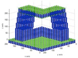
6. •voxel 6° has 1802 points (in green in the picture below).
   

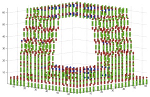
Figure 4. Voxel distribution

At the end of this procedure, the optimal order voxel is found with its amplitude in X, Y and Z .  In this specific case, the parameters produced are:

1. •Optimal voxel: 6°;
   

2. •X amplitude: 3.125;
   

3. •Y amplitude: 3.125;
   

4. •Z amplitude: 3.984.
   

3. CONTOURS

The second procedure is devoted to checking the data set, to analyzing clusters vertically and horizontally, to preliminarily distinguishing chains from sowns and to generating relational matching.

The input file could be CCTV.txt or CCTV_rid.txt. In this case, CCTV.txt is used because in the initial data set there are no double points or points out of height. When there are outliers, the file used is CCTV_RID.txt and not the initial data set.

The input data set is listed with the point ID and X, Y and Z coordinates for each points.

The point ID can be the name of the point or the position in the list: both are used and listed.

The output files are:

1. •CCTV_ord.txt;
   

2. •CCTV_intermediate.txt;
   

3. •CCTV_assemby.txt.
   

The service file is CCTV_connections.txt

The data set can be processed in two different ways:

1. •by checking the input;
   

2. •by checking the data set and analyzing it in terms of clusters and relational matching.
   

The data set is checked in terms of planimetric distance. If points are too close together, only one of them is kept. After this checking procedure, the data set is analyzed.

Input coordinates could be supplied in all possible combinations (X, Y and Z; X, Z and Y; …), the order chosen is 123 (X, Y and Z).

Input data set can also be scaled and rotated, the adopted scales are:

1. •+1.000 in X axis;
   

2. •+1.000 in Y axis;
   

3. •+1.000 in Z axis.
   

and the adopted rotations are:

1. •0 in X axis;
   

2. •0 in Y axis;
   

3. •0 in Z axis.
   

The estimation of the three values needed (the height step between points at consecutive levels, the planimetrical distance between points at the same level and the planimetrical tolerance between points at consecutive levels) is done using “voxel” procedures. The parameters adopted in “contours” procedure are:

1. •height step: 8.000;
   

2. •planimetric distance: 15.000;
   

3. •planimetric tolerance between points at different levels: 4.000
   

The height step parameter, estimated using the “voxel” procedure, is necessary to do vertical clustering.

For each level, the information is listed in this way:

1. •vertical cluster ID;
   

2. •number of points belonging to that level;
   

3. •level;
   

4. •point IDs at that level;
   

The extract of the vertical clusters list is the following:

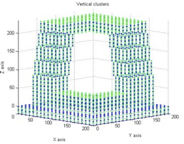
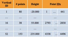
Figure 5 and 6.  Vertical clusters

Here only two 2D plots are attached:

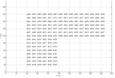
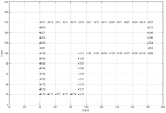
Figure 7.  Two of the 52 vertical clusters

The planimetric distance parameter, estimated using the “voxel” procedure, is necessary to do horizontal clustering. In order to generate contours, finite point sets at each level must be constructed.

These sets could involve all points belonging to a vertical cluster, or there could be different horizontal clusters at the same level, if necessary. This second case is displayed well in the picture below.

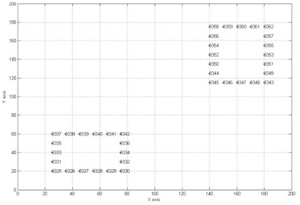
Figure 8.  Two horizontal clusters are needed

Each horizontal cluster is described by:

1. •its horizontal cluster ID level;
   

2. •the number of points that belong to the level clustered;
   

3. •its level;
   

4. •the point ID that belongs to the level clustered;
   

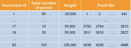
Figure 9.  Procedure output

At level 55.000 there are two horizontal cluster: this is the case in which two different sets are done at the same level. There are 83 horizontal clusters.

The preliminary distinction between sowns and chains is made considering firstly the number of points and secondly, and in the case of ambiguity, the local density.

Generally, points that belong to sowns are denser than the ones that belong to chains. If the number of points is the same, it is necessary to check the local density.

The 3D plot is the following:

Figure 10.  Preliminary distinction between sowns (in green) and chains (in blue)

Although it is a preliminary distinction, all clustered levels are correctly classified, except height 45.000 which is classify as a chain instead of a sown.

The information is listed in this way:

1. •horizontal cluster ID;
   

2. •type of horizontal cluster;
   

3. •vertical cluster ID.
   

At this point, the data set is analyzed in terms of relational matching and the planimetric tolerance parameter, estimated with the “voxel” procedure, is used.

As shown in the picture below, if the relational matching is non-correct, the 3D reconstruct is false and the model adopted is non-consisting.

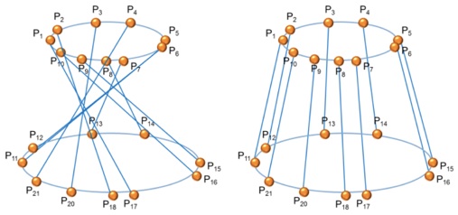
Figure 11.  Incorrect and correct matching

The connection must satisfy the following properties:

1. •the points in question must be as close as possible while still belonging to consecutive levels;
   

2. •if points belong to the same vertical, they are easily matched;
   

3. •if not, we look to create connections along the same direction. For example, in the right picture this last properties is adopted.
   

The relational matching is done separately for chains and for sowns. The former is classified by:

1. •relational matching ID (between one chain and another);
   

2. •horizontal cluster level ID matched to the other horizontal cluster level ID;
   

3. •level matching the other level;
   

4. •the number of points belonging to that matching;
   

5. •the point ID matched to the other or others point(s) ID;
   

The following image shows the output provided.

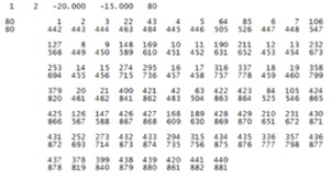
Figure 12.  Relational matching for chains

The latter is classified by:

1. •relational matching ID (between the sown and a chain);
   

2. •horizontal cluster level ID matched to the other horizontal cluster level ID;
   

3. •level matching the other level;
   

4. •the number of points belonging to that matching;
   

5. •the point ID matched to the other or others point(s) ID;
   

6. •the number of sides matched.
   

In this specific case, there is a perfect correspondence between each points so the matching type is a one to one  and the ID point is related to a single point ID.

The total number of sides is also available. In the reconstruction of CCTV, the chain sides matched are 148, the sown sides matched are 18 and the total number is 166.

The specific results are omitted for brevity.

4. CLOSED PATHS

The third procedure is devoted to building closed paths between all chains and all their projections on sowns.

The input files needed are the ones generated in “contour” procedures and are:

1. •CCTV_ord.txt;
   

2. •CCTV_connections.txt
   

3. •CCTV_assembly.txt.
   

The output files are:

1. •CCTV_closedpath.txt;
   

2. •CCTV_connections_cla.txt;
   

3. •CCTV_contours.txt.
   

The four values needed are the three generated with the “voxel” procedure and the fourth is a switch parameter in order to choose which type of interpolation should be used.

The switch parameter can assume two values:

1. •0, for classic paths;
   

2. •1, for Catmull - Rom paths.
   

In our opinion, if points represent the vertices of the object, it is better to model the closed paths using the classic way; if the structure is smooth, Catmull – Rom is the best way.

The values of the first three parameters adopted in “closed-paths”  procedures are:

1. •height step: 8.000;
   

2. •planimetric distance: 15.000;
   

3. •planimetric tolerance between points at different levels: 4.000.
   

For CCTV reconstruction, this parameter is set at 0 because of the shape of the building.

In the first step, the data set is horizontally clustered, in the second, the data is connected one other and each horizontal cluster is finally classify as a chain or as a sown.

At this point it is possible to generate the closed paths, one for each horizontal clusters previously done.

All the points must be taken only once and all sides, if taken, only once too.

The generation of closed paths, elementary in elementary cases, becomes complex as the shape of the path becomes more complicated. In order to force this procedure, the reconstruction of a four letters (F, G, R and W) was preliminarily performed, starting from the rare points. The next four images show the letters analyzed.

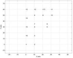
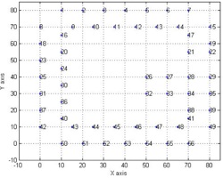
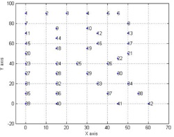
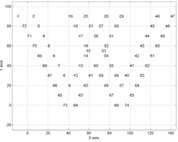
Figure 12.  The four letters analyzed

To find a closed path, first we connect a point to its closest point, next we connect this second point to its closest (excluding the first) and so forth (in order to keep a unique sense of advancement). The sides do not have to cross each other. At this step, a certain number of points will not be connected to the others. Isolated points must be connected in a different hierarchic way:

1. •with the first point, listed in the previous;
   

2. •with the last one, in the same list;
   

3. •with all the remaining points;
   

4. •with all the ones selected, in the meantime.
   

Subsequently, isolated paths are connected. Typically these points belong to levels, separated by a unique level, quite often consisting in one or a few points. Moreover further specific analyses are developed, using to the same mechanism.

Only at this step, it is possible to follow the path of the path. Indeed following a level structure, the path between its root and the farthest leaf identifies the first half of the path. The second part is done attempting to understand if starting from the farthest leaf the root is reached.

In some cases, it is really impossible to reach the root. Therefore, the whole path is formed by adding single steps, starting from the point where the previous step finishes. At the end, when all points have been taken into account, all the sides not used will be deleted, because lying inside the closed path they are useless.

4.1 Piecewise Catmull – Rom’s lines

It is possible to continuously model every path with piecewise Catmull – Rom’s lines and, starting from 3 points, every straight line passes through the second point and it is parallel to the line joining the first and the third points.

The following image shows the Catmull-Rom closed path between 5 generic points.

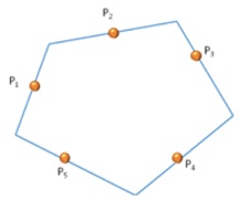
Figure 13.  Perimeter with Catmull – Rom

The advantage of a continuous interpolation is the possibility to extrapolate other points, e.g. intersections between consecutive straight lines.

The output given is divided into two groups: the first one for chains and the second for sowns' contours.

The former are organized as follows:

1. •chain perimeter ID;
   

2. •horizontal cluster ID;
   

3. •side ID;
   

4. •point ID with the ID  of the next point on the perimeter;
   

5. •the total number of perimetred points that belong to chains.
   

The latter (closed paths for the sowns' contour) are  organized as follows:

1. •sowns perimeter ID;
   

2. •horizontal cluster (sown) ID and horizontal cluster (chain) ID;
   

3. •side ID;
   

4. •point ID with other point ID consecutively in the perimetration;
   

5. •the total number of perimetred points that belong to chains;
   

6. •the total number of perimetred points
   

The results of the interpolation in Catmull – Rom perimetretion are divided in contours of chains and contours of sowns. The reports are organized like so:

1. •interpolation ID;
   

2. •horizontal cluster ID;
   

3. •side ID;
   

4. •ID of the three consecutive points on the perimeter;
   

5. •type of straight line
   

6. •y = ax + b
   

7. •y = cy + d
   

           in the first case, a y is displayed while in the second, an x;

1. •the slope of the straight line;
   

2. •y-intercept or x-intercept.
   

The following image is an extract of the interpolation results for the chains.

Figure 14.  Chains interpolation

If Catmull – Rom perimetration is set, the straight lines intersect each other so the “closed-path” procedure lists some additional information, divided for chains and sowns:

⋅ID of the three consecutive points (belonging to chains or to sowns) on the perimetration;

⋅X, Y and Z coordinates of the intersection point;

⋅number of intersected points for chains;

⋅number of intersected points for sowns;

⋅total number of intersected points.

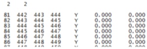
Figure 14.  Chains interpolation

If Catmull – Rom perimetration is set, the straight lines intersect each other so the “closed-path” procedure lists some additional information, divided for chains and sowns:

1. •ID of the three consecutive points (belonging to chains or to sowns) on the perimetration;
   

2. •X, Y and Z coordinates of the intersection point;
   

3. •number of intersected points for chains;
   

4. •number of intersected points for sowns;
   

5. •total number of intersected points.
   

4.2 Classic way

It is also possible to model every path in the classic way, in order to make a comparison between the two modes (Catmull-Rom and the classic way).

The following image shows the classic contour between the same five points displayed in figure 13.

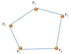
Figure 15.  Classic perimeter

Here two images are attached showing two examples of classic perimeters: the former is for chains and the latter is for  sowns' contours.

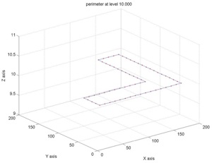
Figure 16.  Classic perimeter for a chain (level 10.000)

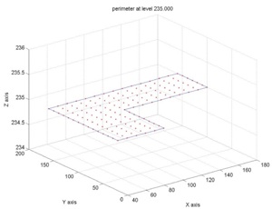
Figure 17.  Classic perimeter for the contour of a sown (level 235.000)

The following image shows the perimetretion done in the classic way:

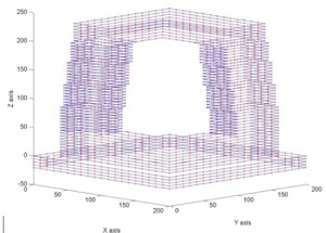
Figure 18.  Classic perimeter

This final distinction between sowns and chains is done considering separately points that belong to connections classify as sowns–chains or sowns–sowns and points that belong to connections classify as chains–chains.

For the former the numbers of points is compared: if the first group is composed of a greater number than the other one, the first is classify as a sown while the second one as a chain. On the contrary, if the first group is composed of a lower number than the other one, the first is classify as a chain while the second one as a sown.

For the latter, first the existence of all sowns or all chains is checked. If it is not so, a cycle begins in order to fix all chains making a comparison between the number of points that belong to subsequently horizontal clusters.

At the end, if there are some connections non-classified, the type is set as a sown.

As shown in the following image, all the clusters are correctly classify.

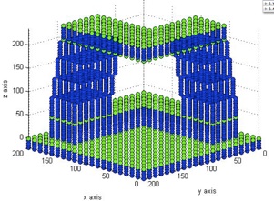
Figure 19. Distinction between sowns (in green) and chains (in blue)

The levels 0.000, 45.000, 205.000 and 235.000 are correctly classify as sowns, all the others as chains.

5. TRIANGLES

The fourth procedure is devoted to connecting points in triangles. These points belong to subsequent chains or subsequent sowns or chains and their projections upon the nearest sowns. There are many possible triangulations, the adopted one is the Delaunay triangulation, where triangles are as equilateral as possible and each triangle must not contain any other points. This last fact implies that a circumcircle passing through three points, should not contain any other point. Delaunay triangulations maximize the smallest of all the angles of the triangles in the triangulation. This triangulation was invented by Boris Delaunay in 1934.

In the Delaunay triangulation of a discrete point set, P in a general position corresponds to the dual graph of the Voronoi tessellation for P.

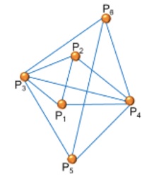
Figure 20.  Random triangulation

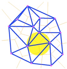
Figure 21. Delaunay triangulation (in blue), Voronoi tessellation (in orange) and circumcircle (in yellow).

The previous picture shows a random triangulation but it is wrong because:

1. •the triangle should be as equilateral as possible;
   

2. •a circumcircle should not contain any of the other points (it is shown in figure 21)
   

3. •the smallest inner angle must be at its maximum breadth
   

If the structure in concave Delaunay triangulation doesn’t work so we make the following adaptation: we check if the middle point of the side of the triangle is inside the closed path, on the perimeter or outside the closed path. If it is inside or on the perimeter, we keep it, otherwise we delete the line.

Figure 22.  Wrong Delaunay triangulation for a concave body

For example. the middle points P11 and P12 in picture 23, are outside the perimeter so sides P7 – P6 and P7 – P2 are deleted.

If the body has a hole, the 3D model must have the same hole. So if a side is found within the hole, it will be deleted.

For example. the middle points P9 in picture 24, is inside the hole so the side P1 – P5 is deleted.

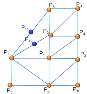
Figure 23.  Wrong Delaunay triangulation for a multi-connected body

The input files needed in the “triangles” procedure are:

1. •CCTV_ord.txt;
   

2. •CCTV_connections_cla.txt;
   

3. •CCTV_assembly.txt;
   

4. •CCTV_closedpaths.txt;
   

5. •CCTV_contours.txt.
   

The output files given are:

1. •CCTV_triangles.txt;
   

2. •CCTV_newpoints.txt.
   

The three values needed are estimated using “voxel” procedures and are:

1. •height step: 8.000;
   

2. •planimetric distance: 15.000;
   

3. •planimetric tolerance between points at different levels: 4.000.
   

The triangulation can connect points belonging to the horizontal cluster, at the same level, as in the extract below:

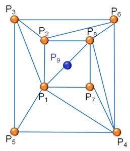
Figure 23.  Wrong Delaunay triangulation for a multi-connected body

The input files needed in the “triangles” procedure are:

1. •CCTV_ord.txt;
   

2. •CCTV_connections_cla.txt;
   

3. •CCTV_assembly.txt;
   

4. •CCTV_closedpaths.txt;
   

5. •CCTV_contours.txt.
   

The output files given are:

1. •CCTV_triangles.txt;
   

2. •CCTV_newpoints.txt.
   

The three values needed are estimated using “voxel” procedures and are:

1. •height step: 8.000;
   

2. •planimetric distance: 15.000;
   

3. •planimetric tolerance between points at different levels: 4.000.
   

The triangulation can connect points belonging to the horizontal cluster, at the same level, as in the extract below :

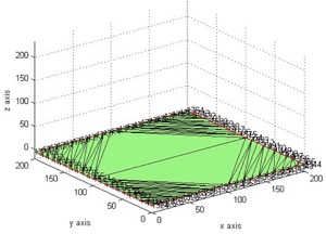
Figure 24.  Delaunay triangulation
(level -5.000)

Each triangulation is associated with a Voronoi tessellation.

The Delaunay triangulation is also applied to points that belong to a different level. This is done in order to create a rough 3D surface.

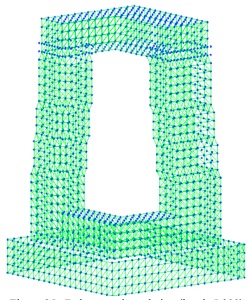
Figure 25. Delaunay triangulation (level -5.000)

6. BÉZIER SPLINE

The fifth procedure, still being implemented, is carried out using one of our own softwares called “tri_spline”, is devoted to interpolating triangles with triangular splines. For this task, the Bézier spline is used, because it forms continuous surfaces with one continuous derivative surfaces.

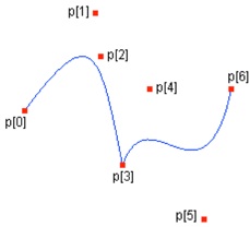
Figure 26.  Two splines connected in the middle point

The reconstruction becomes smoother, even if surface breaklines are accepted. Notice that discontinuities of second derivatives are geometrically a bit less evident and therefore neglected.

It is necessary to point out that it is difficult to identify breaklines not highlighted in the input. Another theoretical problem is the analytical complexity of the solution, because the pair of coordinates, which should be used instead of the one dimensional curvilinear coordinate, is not yet globally defined.

At the moment, some theoretical aspects should be studied in detail, recognizing the elegance of the Bézier spline, even in one-dimensional space.

7. FUTURE WORKS

The estimates of the first three parameters done using the “voxel” procedures are an underestimation of the real values.

The second problem to be analyzed is the possibility to model  almost-horizontal sowns correctly. In this specific case, the top of CCTV is not horizontal, while in the 3D model it is analyzed and treated as a horizontal plan.

The third problem is the fact that the Bézier spline is well known, but there is no definite coordinate pair so some extra studies are needed in order to find a solution.

8. COMMENTS

Our first comment regards the results as a whole: they try to take a step forward compared to a wide range of previously collected samples. In any case, all programs (except for computer graphics applications) are written, implemented, tested and used forming a library of our own softwares.

The second comment relates to the approach used: the user is provided a graphic result and *.txt files where all the results are analyzed.

REFERENCES

George A. Liu Jwh, 1981. Computer solution of large, sparse, positive and definite system, Prentice all, Engliwood Clifts, New Jersey.

Hawkins D.M.,  1980. Identification of outliers, Chapman and Hall, London.

Jodidio P., Architecture now!, volume 7, 2010.Taschen.

Kaufman L. Rousseeuw Pj, 1990. Finding groups in data, Prentice all, Engliwood Clifts, Wiley&Sons, New York.

Morteson Me, 1997. Geometric modeling, Wiley&Sons, New York.

Naldi G., Pareschi L., 2007. Matlab, concetti e progetti. Apogeo, Lavis (TN).

Preparata F. P., Shamos M. I., 1985. Computational Geometry, an Introduction, Springer, New York.

Thurston W., 1997. Three-dimensional Geometry and Topology, Princeton University Press, Princeton.

Week J., 1985. The shape of space, Dekker, New York.